Detecting eggs in the nest
- Par arnaudawelty
- Le 18/01/2017
- Dans Prototype
The Eggs-iting Smart Chicken Coop should be able to accurately count the number of eggs in the nest and notify you directly on your app. This information is at the heart of the future apps on Eggs-iting, putting the chickens and the eggs first..
Living conditions
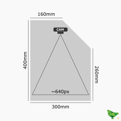
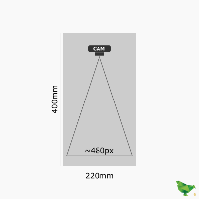
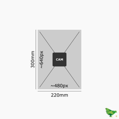
One of the essential features of the Eggs-iting Smart Chicken Coop is to notify instantly when a new egg is laid. We selected a detection system from a low-resolution camera (webcam) positioned to watch the nests.
The nests inside the chicken house do not have natural daylight, so a LED light source illuminates the scene to be photographed. The power and duration of lighting must not impair the comfort of the animals or cause excessive energy consumption.
The entire chicken coop is driven by a Raspberry Pi robotic system using Debian Jessie Lite. The camera is connected directly to the USB port. The lighting is controlled by the GPIO outputs of the board whose logic outputs are transmitted by power transistors.
| Camera resolution | 640 x 480 |
| LED Lighting Power | 0.2A sous 5V / 1W |
| LED Turn on time | 5 seconds |
| Nest width | 22 cm |
| Nest depth | 30 cm |
| Nest height | 40 cm |
Characterization of an egg
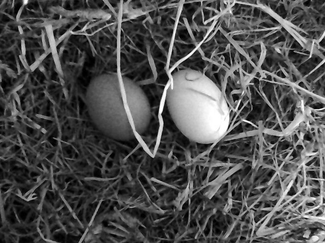
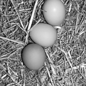
A nest can accommodate up to a dozen eggs of different sizes, colors and practically identical shapes. None of these characteristics are ;sufficiently stable to be systematically sought out.
See opposite photo, two eggs of different sizes and colors.
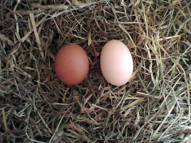
By color
The color of an egg may vary depending on several biological factors (species, diet, health status of the hen), and may differ from the colors on the camera. Consumer sensors and the electronics that accompany them carry out automatic calibrations (exposure, white balance) on the whole scene. The color tracking approach was therefore quickly eliminated.
By surface area
Straw, hay, feathers or dirt can partially cover the eggs, preventing the identification of homogeneous surface area of the eggs. A first approach to detect surface area was attempted.
From a grayscale version, the contours are detected(type Laplace), then an expansion makes it possible to eliminate the majority of the unrelated noise (like straw or hay). A threshold is finally applied to isolate the "united" zones.
Attempt to detect surface area


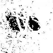
As observed the strands of straw "cut" the egg in several zones. It is difficult, a posteriori, to collect these areas and to associate them with their original surface.
From the average surface of an egg, however, we could calculate the approximate number of eggs, regardless of the shape or position of the detected areas.
By geometry
An egg can also be partially hidden by another if the eggs are touching or overlapping. Eggs position can also be standing at different angles or laying on its side.
Geometric detection (Circle Hough Transform (CHT)) is therefore relatively expensive, since it must look for potentially incomplete and arbitrarily oriented ellipses.
By gradient
In addition to the shape and color of the eggs, their spherical properties can be exploited. Since a fixed light source is available, and the eggs are essentially ovoid, one can bet on an even light distribution from one egg to another.
By measuring gradients between each pixel and its neighboring egg, one should be able to observe an identifiable pattern.
Local Binary Patterns(LBP) have been defined with the objective of identifying repeating patterns in an image. Mainly used to detect and recognize textures, they can be exploited locally to recognize contours, corners, or shapes.
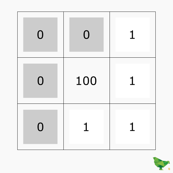
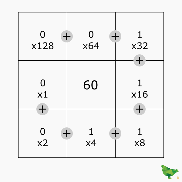
Method of Local Binary Pattern calculation
To calculate the "LBP derivative" of an image, one proceeds in the following way:
- For each pixel p of the image having 8 neighbors
- Let an 8-bit LBP value numbered b0 to b7
- For each of the 8 neighbors v (0 to 7) of the pixel in question, clockwise
- Calculate the difference in intensity between this neighbor v and the pixel p
- If the difference is positive, set the corresponding LBP bit to 1
- Otherwise set the corresponding LBP bit to 0
Example of Local Binary Pattern convolution
From left to right:
- Initial image
- Grayscale image
- LBP derivative


How to use the LBP
After tests on around a hundred images, we note that the eggs, once "derived", all have approximately the same distribution of values. We will exploit this characteristic from local histograms as a set of reference images.
To perform the test groups one selects a dozen reference images, cropped to the nearest objects to be searched.

The LBP of each test image is calculated and a normalized local histogram is extracted for each of the 4 quadrants (histA, histB, histC, histD) of the image.
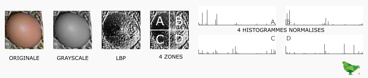
Once the 12 images are processed, the average of the histograms is calculated for each of the 4 corners. We obtain 4 normalized histograms (avgA, avgB, avgC, avgD), which present the average distribution of the values for each of the 4 corners of the image sought.
Finding objects in an image
From the image, then we go through it with a window whose size is close to the objects to be searched. The dimensions of the window must be divisible by 2.
We extract the 4 histograms (kingA, kingB, kingC, kingD) from this window, and compare them to the average histograms (avgA, avgB, avgC, avgD). The obtained score is stored in a matrix of the same dimensions as the image analyzed.
Since we compare standardized histograms, the number of pixels used for training or analysis does not matter, it is the distribution of values that is compared, not the values themselves.
The difference between 2 histograms is obtained from the Chi-square method. Given two histograms A and B, the delta difference between the two is calculated as follows:
Δ = ∑( (a-b)² / (a+b) )
Two "similar" histograms will be considered if the delta obtained is less than a chosen threshold defined as S. The observed window score is the number of corners with a delta lower than S.
The number and position of the detected objects is obtained by isolating the maximum scores.
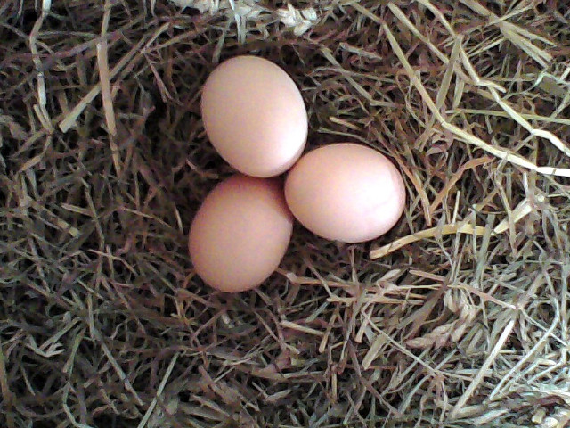
Illustrative analysis of an image
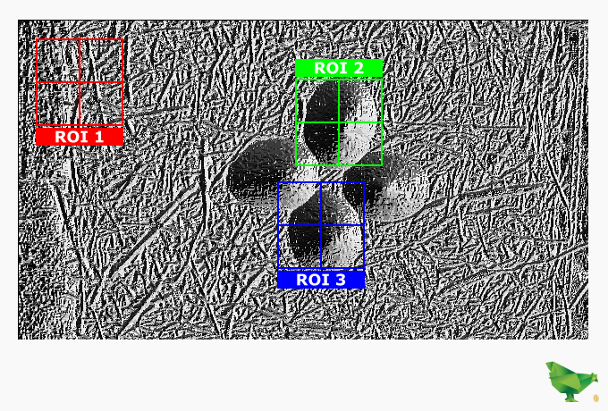
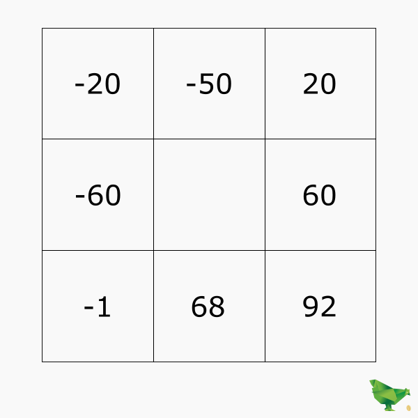
Calculation of scores with an acceptance threshold of 160
| Zone | deltaA | deltaB | deltaC | deltaD | Score |
| ROI 1 | 450 | 524 | 496 | 536 | 0 |
| ROI 2 | 142 | 121 | 92 | 102 | 4 |
| ROI 3 | 217 | 105 | 148 | 154 | 3 |
- Zone 1 obtains a zero score because none of the quadrants of the image presents a histogram close to that realized during the testing.
- Zone 2 obtains the maximum score of 4 because the histograms of the 4 quadrants are sufficiently close.
- Zone 3 has a score of 3 because the histogram in the upper left corner is not retained. (Because of the left egg encroaching on this quadrant)
Tests and results
On a test set of 100 images, showing 0, 1, 2, 3 or 4 eggs (with a total of 200 eggs), this method achieved a 100% success rate.

